Predicting NBA Career Performance Based on Rookie Season

Introduction

What are we trying to accomplish?

Forecast a player’s career win shares (number of wins attributable to a player) per season based on their rookie metrics.

Why is it important?

NBA teams win or lose games based on the number of win shares their players create. Being able to predict the career performance of a player in their rookie season is important to team management because it allows them to make better draft, trade, and personnel decisions to give their organization the best opportunity of winning a championship.

Data

Where did we get the data?

Source: https://www.basketball-reference.com/

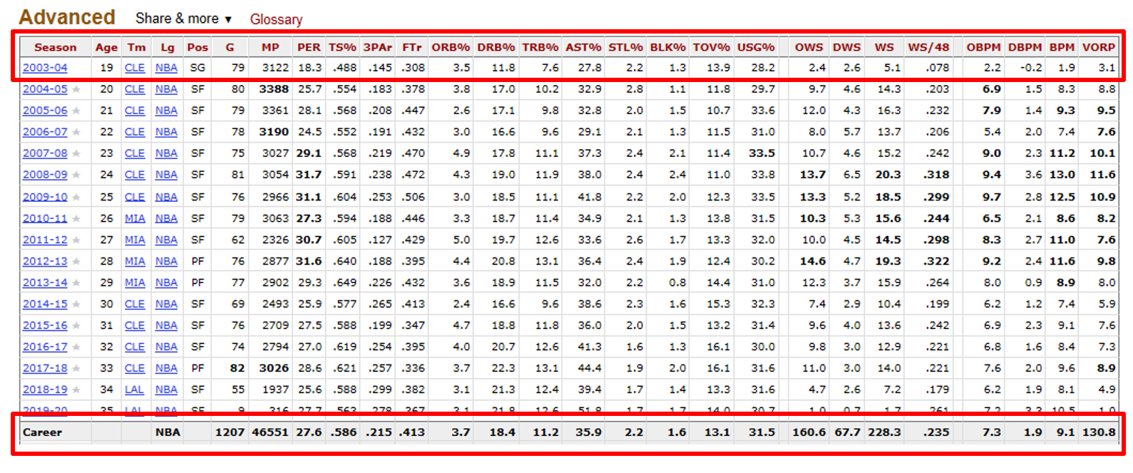
What are its characteristics?

All players who were rookies between 1980 through 2018 were included in the dataset.
Each row (2,217) corresponds to an individual player.
The features include 23 rookie metrics and 20 career metrics.
Features include information about player efficiency rating, true shooting percentage, 3 point attempt rate, free throw attempt rate, rebound percentage, block percentage, assist percentage, steal percentage, etc. (see Appendix - Glossary of Features)

What is Our Approach?

The approach was 2 fold as below.

Unsupervised

We used clustering analysis to find groups of seasoned players (10+ years in the NBA) to which to compare rookie players. To do this we found 2 new features, using Linear Discriminant Analysis (LDA), that reduced the dimensions of the rookie and career features into single metrics. These new features were correlated with rookie and career win shares, and used for clustering analysis.

Supervised

We used supervised learning to predict the career win shares of a player by using their rookie data. We went through different analysis approaches to pick the most important features in the rookie matrix. Furthermore, these features were used by various models. We also chose the best model by comparing the RMSE, R-squared and Mean Absolute Error values generated by these models.

What is new in our approach?

Using LDA to create new features that reduced the dimensions of the rookie and career features into single metrics, and then using these metrics to predict career performance is novel in our approach.

We also used Huber regression, elastic net, and gradient boosting to predict career win shares per season. In our research, we did not see anyone use these approaches to predict a rookie's career outlook.

Unsupervised

Creating new features

Created a new variable, rookie win shares classifier. This variable had a value of 0 if the player’s rookie win shares were 1 standard deviation below the mean, 1 if the player’s rookie win shares were within a standard deviation of the mean, and 2 if the player’s rookie win shares were 1 standard deviation above the mean.
For players who were not rookies in 2018, we created a similar metric for normalized career win shares (divided by number of years played in the NBA).
Using the rookie win shares classifier as a label, we used LDA as a dimension reduction technique to find a linear combination of the rookie features that were predictive of rookie win shares.
We also created a LDA model for normalized career win shares.
The first component of the rookie LDA model and the first component of the career LDA model were used as a new set of features for clustering analysis. The first components were chosen because they are the features most responsible in their models for maximizing win share class separability.

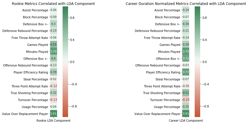
LDA features and original features correlations

The following plot shows how the original rookie and career features are correlated with the values of the chosen LDA components.

9 classes

With the 2 new components derived from the 2 LDA models, we plotted all NBA players since 1980 who were not rookies in 2018, with their respective labels.

The x axis corresponds to the value of the first component that was derived from the LDA model for duration normalized career win shares.
The y axis corresponds to the value of the first component that was derived from the LDA model for rookie win shares.
The colors correspond to the original 0 (Bad), 1 (Avg), and 2 (Good) classification values created in the career (C) and rookie (R) win shares classifier variables. Combinations of the original 2 classification variable values creates 9 total classes.

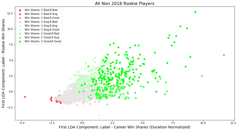
This plot shows that the two LDA are positively correlated with each other, and they are positively correlated with rookie/career win shares.

Seasoned players: 6 classes

Rather than compare 2018 rookie players to other players who have had a few years in the league, it is more interesting to compare rookies to players who have had long careers in the league; there is more information about these players. In this spirit, we reran the LDA analysis for players with 10+ years in the league. The following plot shows the results of this analysis.

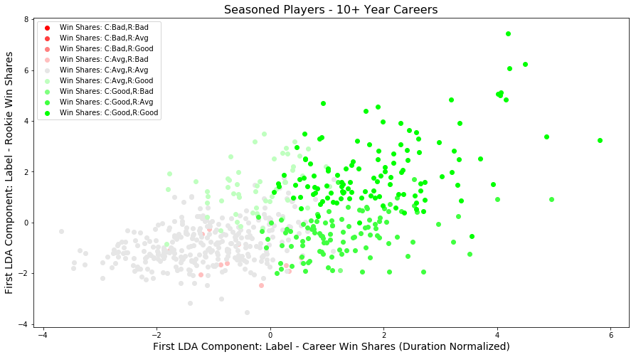
Only focusing on seasoned players (10+ year NBA careers) reduces the number of classes represented from 9 to 6; there are not many seasoned players with low career win shares per year. Those types of players usually don’t make it 10+ years in the league.

Clustering

Because we know seasoned players represent 6 unique classes, we chose to use clustering algorithms that resulted in 6 clusters. In K-means and GMM we explicitly set the number of cluster centers equal to 6. In hierarchical based clustering we pruned the dendrogram to have 6 clusters. In DBSCAN we adjusted epsilon and min points such that 6 clusters resulted. The following sections show the results of each clustering method used. We then provide an evaluation of the 4 clustering methods.

Kmeans

For K-means we initialized centers 25 times and picked the clustering that minimized within cluster distances and maximized between cluster distances. The graph below depicts the 6 resulting clusters. Hall of Fame players with amazing rookie seasons, such as Allen Iverson, were clustered in the upper right portion of the graph, while less accomplished players such as Vitaly Potapenko appeared in the bottom left of the graph. The players listed in the center of their clusters represent the players closest to their cluster’s mean.

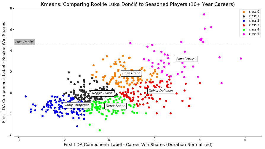
Comparison of rookie players to seasoned players

To compare rookie players from the 2018 season to players with 10+ years in the league, we used the seasoned player’s rookie LDA model to get component values for 2018 rookie players in 2018. We then plotted rookie players on a line, on the y axis, at this value.

In the plot above, for example, Luka Dončić, has a LDA component value from the seasoned rookie LDA model of 4.73, highest among 2018 rookies. If Luka plays for 10+ years in the league, his career metric would be plotted along the gray line. Although, it is possible for him to end up in the blue, black, or orange cluster (unlikely because no player with his rookie performance has before been included in these clusters), Luka will most likely be included in the pink cluster (where many greats of the game are located).

This information is useful to the Dallas Mavericks, Luka’s current team, because it helps them know how to value their player.

Gaussian Mixture Model

GMM is a soft classifier, where every point has a probability of being included in a cluster. Points were assigned to clusters based on its maximum probability across all its probabilities of belonging to a certain cluster.

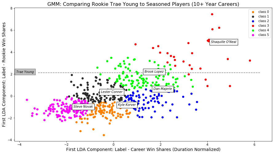
The clustering results appear similar to Kmeans, however, some of the players located closest to their cluster means are on the periphery of the soft assignments.

This plot shows that Trae Young (who ironically the Atlanta Hawks traded for by trading away Luka) will most likely be in the green cluster with Brook Lopez. However, there is a chance he could also end up in the black or red clusters.

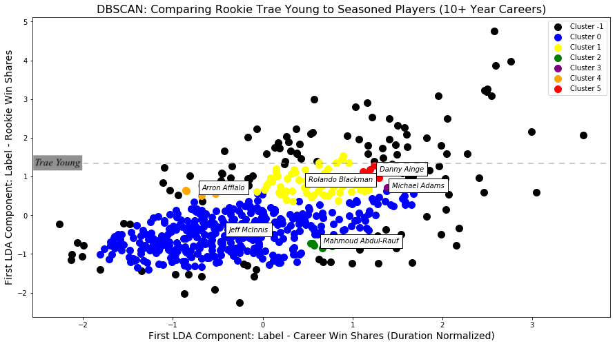
DBSCAN

Unlike other clustering algorithms, DBSCAN does not require to specify the number of clusters a priori. The number of groups depends on two parameters: epsilon (the distance from a given point) and min points (the minimum number of points within epsilon to be considered a cluster). After adjusting the values of epsilon and min points, six clusters were identified. The white labels show players who were closest to the center of their clusters. The black dots represent players who are regarded as outliers (indicated as cluster -1). For example, data points in the upper right corner are spread out or are not dense enough to be clustered. There are many exceptional players who are located in this region of the graph.

If Trae Young plays 10+ seasons, he could fall under Cluster 1 (yellow), Cluster 5 (red), or become a noise point.

Hierarchical

In hierarchical clustering, a dendrogram was used to cluster players. Below is the dendrogram diagram. The x-axis consists of the players and y-axis consists of the Euclidean distance between the clusters. While there are many distance measuring methods (e.g. single, complete, average, ward, etc.), we used average method to best match our pre-existing classes (see evaluation section for more details). As the dashed line indicates, we cut the dendrogram at approximately 1.6 to obtain 6 clusters.

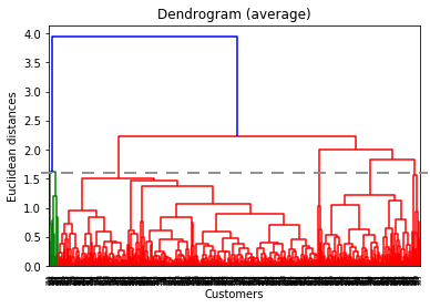
Below is the hierarchical clustering results. The most noticeable difference between K-means/GMM and Hierarchical clustering is observed in Cluster 2 (indicated as green color). While K-means and GMM separated Cluster 2 as two or more groups, hierarchical clustering clustered them as one group, which is similar to our pre-existing categorization of seasoned players.

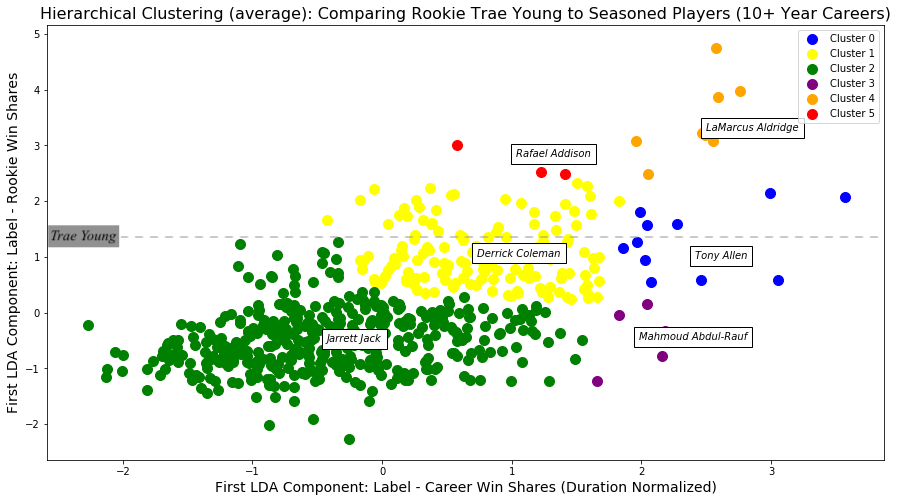
Trae Young can potentially belong to three different groups: Cluster 0 (blue), Cluster 1 (yellow) and Cluster 2 (green). Young will most likely belong to Cluster 1.

Evaluation of clustering methods

Since we know the 6 labels of our seasoned players, we evaluated our clustering using Adjusted Rand Index (ARI) score. The score values for each clustering technique are the following:

K-means:0.29
GMM:0.34
DBSCAN:0.34
Hierarchical:0.40

The ARI is calculated by the number of pairs of components that are either in the same group or in different groups divided by the total number of pairs of components. The maximum value 1 and the minimum value 0. A higher value of adjusted ARI means a higher match between two groups. The ARI can also measure agreement between two different cluster groups even though they have different indices of clusters.

While the ARI score does not determine the best clustering algorithm, it gives the similarity value between two clustering indices. As indicated in the above table, the clusterings using hierarchical method are the most similar to the original clustering groups. The visual comparison between the hierarchical clustering result and the 6 classes of seasoned players allows us to identify two major groups: Cluster 1 (yellow) and Cluster 2 (green).

Supervised

Exploratory data analysis

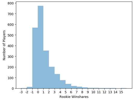
Before further discussing the project, we used basic EDA to see what our data could tell us. First, we looked at the distribution of rookie win shares:

Next, we looked at career win shares:

We can see that the distribution of win shares is skewed to the right. This makes sense since the very good NBA players have very high win shares. For example, the win shares leader of our data set is Karl Malone, with 234 win shares. So, it’s an elite status to have a high win shares.

Furthermore, by comparing the 2 charts, we realize that the range of career win shares is lot bigger than the rookie win shares. This makes sense since the career win share values are created by adding the win shares of a player during their career. This observation resulted in our approach to take into consideration the “duration” of career, while calculating win shares.

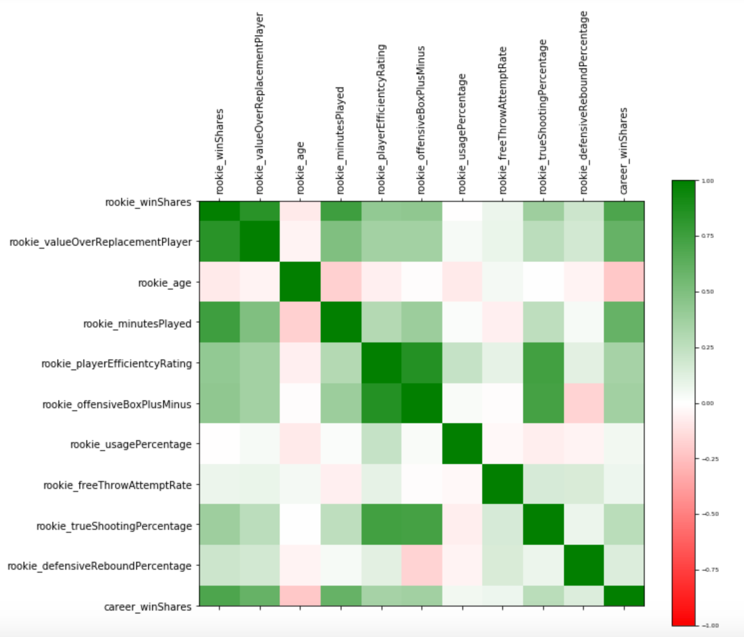
We have calculated the correlation of all the attributes with the career win shares. This plot shows the attributes that are highly correlated with this metric.

Modeling and Insights

Regression using LDA components

For our first approach, we trained various models using the LDA components obtained from the unsupervised analysis. In this approach, we used LDA on rookie features of all non-rookie players. Then, we used took the first 2 LDA components and used them in various models. We looked at the accuracy of each model using 5-fold cross validation on non-rookie players and their corresponding career win shares. The following table shows these results:

Regression and regularization models using rookie features

Win shares is a continuous variable; we used linear regression to predict career win shares per season. We also scaled the attributes, as few values have different quantities which would impact the linear regression algorithm. Below is a chart of important attributes using linear regression. This chart shows the strength of coefficients of each predictor.

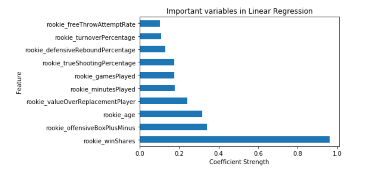
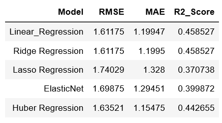
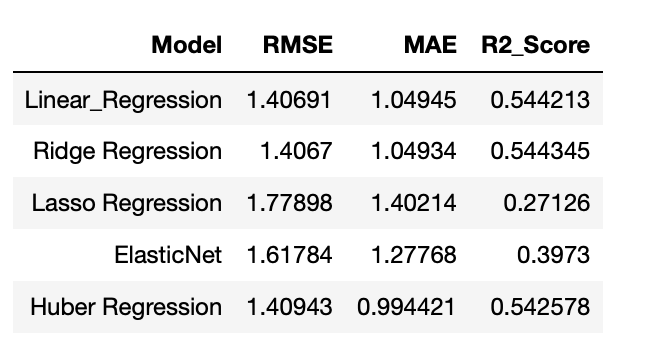
Our experiments include regularizing linear regression algorithm with ridge(L2 norm), lasso (L1 norm) and elastic net techniques. There are outlier values in our data. To handle such outliers in the player stats we experimented with Huber loss in linear regression. This model handles outliers well by minimizing the contribution of outliers to the loss function.

The below chart compares various techniques in linear regression. We used RMSE, MAE, R-squared for evaluating the models.

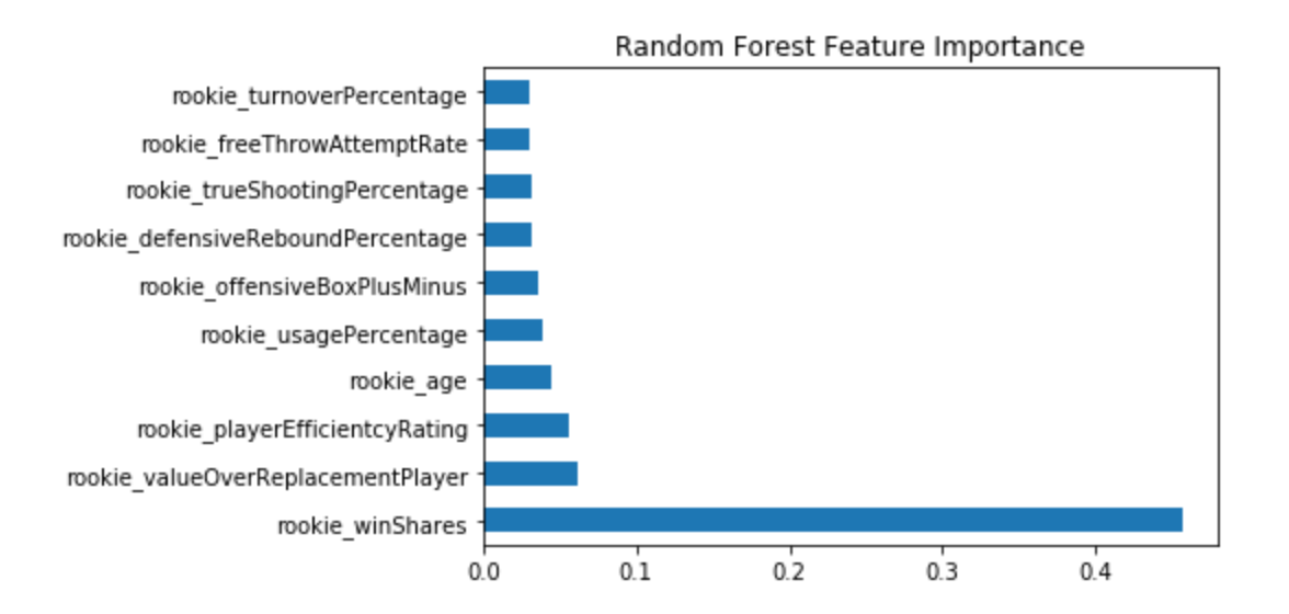
To further improve the model, we trained a random forest regressor with hyperparameter tuning using 5-fold cross validation technique. The chart below shows the important features in the random forest model.

We also trained boosting algorithms, such as the gradient boosted tree regressor. This gives similar performance compared to other models explored. Below chart compares various models.

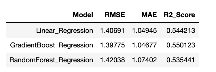
Many of these models were comparable in predictive performance. Gradient boosted regression gave the best RMSE at 1.39, while Huber regression gave the best MAE at .99.

Career win share per season prediction for rookies

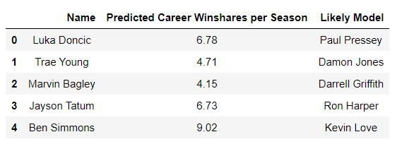
Above is an image of top rookies from 2017-2018 season and 2018-2019 season, including Atlanta Hawk's Trae Young. These rookies' career win shares per season were predicted using rookie features via linear regression. Then, their prediction was matched with a career win shares per season of players who have played 10 or more years in the NBA. If there were multiple matches, a player in roughly the same position was picked (i.e. guard to guard). For Ben Simmons, Kevin Love as well as Amare Stoudemire were matches. It was interesting to see that Ben Simmons was comparable to these two "big men".

Conclusion

For unsupervised learning, hierarchical clustering provides the best performance relative to actual labels. Clustering using LDA components gave us the ability to compare 2018 rookies to seasoned NBA players.

For supervised learning, three models that were explored, linear regression, random forest regression, and gradient boosting. All provide similar performance, but gradient boosting and Huber regression gave the best results. Linear regression shows that the top three most important features in predicting career win shares per season are rookie career win shares, rookie offensive box plus minus, and rookie age. In addition, dimensionality reduction was done using LDA and its outputs were used as inputs for various models. However, this did not improve predictive performance.

Appendix

Glossary of features

year: the year the player started their rookie season. (rookie)
age: age of the player on February 1st of their rookie season. (rookie)
team: the player’s team their rookie season. (rookie)
position: what position the player played their rookie season. (rookie)
games played: number of games played. (rookie/career)
minutes played: number of minutes played. (rookie/career)
player efficientcy rating: measure of per-minute production standardized such that the league average is 15. (rookie/career)
true shooting percentage: measure of shooting efficiency that takes into account 2-point field goals 3-point field goals and free throws. (rookie/career)
three point attempt rate: percentage of field goal attempts from 3-point range. (rookie/career)
free throw attempt rate: number of free throw attempts per field goal attempt. (rookie/career)
offensive rebound percentage: estimate of the percentage of available offensive rebounds a player grabbed while he was on the floor. (rookie/career)
defensive rebound percentage: estimate of the percentage of available defensive rebounds a player grabbed while he was on the floor. (rookie/career)
total rebound percentage: estimate of the percentage of available rebounds a player grabbed while he was on the floor. (rookie/career)
assist percentage: estimate of the percentage of teammate field goals a player assisted while he was on the floor. (rookie/career)
steal percentage: estimate of the percentage of opponent possessions that end with a steal by the player while he was on the floor. (rookie/career)
block percentage: estimate of the percentage of opponent two-point field goal attempts blocked by the player while he was on the floor. (rookie/career)
turnover percentage: estimate of turnovers committed per 100 plays. (rookie/career)
usage percentage: estimate of the percentage of team plays used by a player while he was on the floor. (rookie/career)
win shares: estimate of the number of wins contributed by a player. (rookie/career)
offensive box plus minus: box score estimate of the offensive points per 100 possessions a player contributed above a league-average player translated to an average team. (rookie/career)
defensive box plus minus: box score estimate of the defensive points per 100 possessions a player contributed above a league-average player translated to an average team. (rookie/career)
box plus minus: box score estimate of the points per 100 possessions a player contributed above a league-average player translated to an average team. (rookie/career)
value over replacement player: box score estimate of the points per 100 TEAM possessions that a player contributed above a replacement-level (-2.0) player translated to an average team and prorated to an 82-game season. (rookie/career)
duration: how many years the player paid/has played in the league.(career)
id: the unique identifier of the player

Distribution of work

Data scrapping and cleaning: Cameron Bradley
Unsupervised feature engineering: Cameron Bradley
Supervised feature engineering: Kalyan Murahari
Linear regression and regularization: Kalyan Murahari, Kevin Cho
Exploratory data analysis: Nazanin Tabatabaei, Kalyan Murahari, Kevin Cho
LDA for supervised models:Nazanin Tabatabaei
Random Forest, Gradient Boosting: Kalyan Murahari
Rookie prediction match: Kevin Cho
Kmeans and GMM: Cameron Bradley
DBSCAN and Hierarchical: Sungeun An
Clustering evaluations: Sungeun An
GitHub page contributer: Cameron Bradley, Sungeun An, Nazanin Tabatabaei, Kevin Cho, Kalyan Murahari
GitHub page editor: Cameron Bradley, Nazanin Tabatabaei